Sub-resolution gap extraction from ARPES
Condensed-matter physics · advised by Prof. Yu He, Yale Applied Physics · 2021–2023
The standard way to measure a superconducting energy gap from photoemission is to fit a single curve: one energy slice at the Fermi momentum. When the gap is smaller than the instrument’s energy resolution, that single slice blurs two peaks into one and the fit falls apart. Working in Yu He’s lab at Yale, I built a method that fits the whole band instead of one slice: two rounds of simple fits that read the gap off the dispersion’s shape. Below the resolution limit it cut fit residuals several-fold, up to ~20×, and ran in under a minute where a full 2D fit took hours. It won 2nd place at a Berkeley Advanced Light Source user meeting.
The gap you can’t resolve
In a superconductor, electrons below a critical temperature pair up and open an energy gap: a forbidden band of energies right at the Fermi level. Measuring how that gap opens and closes as you change temperature, momentum, or doping is one of the most direct windows we have into why a material superconducts. Angle-resolved photoemission spectroscopy (ARPES) is the tool of choice: shine light on the sample, measure the energy and angle of the electrons that come out, and you get a 2D map of intensity over binding energy and momentum: the band structure, directly.
To read the gap off that map, the textbook recipe takes a single vertical slice, an energy distribution curve (EDC), at the Fermi momentum k_F, symmetrizes it about the Fermi energy, and fits it. k_F is the natural choice: it’s where the band moves the most, and where particle–hole symmetry lets you symmetrize away the messy Fermi cutoff. A gapped EDC shows two peaks straddling the Fermi energy, split by roughly twice the gap.
Resolution is what makes this hard. When the gap Δ shrinks below the analyzer’s energy resolution, those two peaks smear into a single blob, and a single-slice fit can no longer tell a small gap from no gap at all, exactly the regime you care about near a phase transition. Drag the sliders below: shrink the gap or coarsen the resolution and watch the left panel, a single EDC at k_F, lose the two-peak signature entirely.
k_F: grey is the intrinsic lineshape, blue is what the analyzer actually records, and the rust ticks mark the true gap at ±Δ. That two-peak split is what a single fit relies on. Right: each dot is one EDC’s fitted peak position, and the teal curve is the dispersion fit; its closest approach to the Fermi level is the gap. An illustration of the exact model the study fits, not the study’s data.Use every EDC, not just one
First, the peak-overlap problem is worst right at k_F: as temperature rises, the peaks from the lower and upper bands overlap there first. A little to either side of k_F, the peaks stay separated to higher temperatures and smaller gaps. Second, the conventional recipe throws away almost all of the data: a full ARPES map has hundreds of EDCs, and it fits exactly one. The EDCs near k_F carry nearly the same information; they’re just conventionally ignored.
So rather than trust one slice, use the whole neighborhood. The gap doesn’t only live in the splitting of a single EDC; it lives in the shape of the band. A gapped band bends back before it reaches the Fermi level instead of crossing it, and the size of that back-bend is the gap. That’s something you can measure from the collection of peak positions across momentum, even when no single EDC can resolve the splitting on its own (the right panel above).
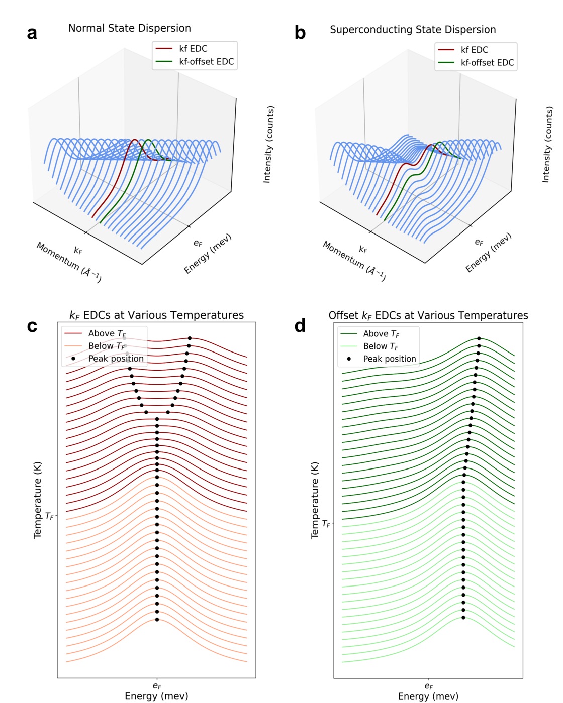
k_F keeps working longer. (a, b) EDC-stack schematics of the band: in the normal state (a) the dispersion crosses the Fermi energy; in the superconducting state (b) it bends back before reaching it, and the size of that back-bend is the gap. The red curve is the EDC at k_F, the green curve one at a small momentum offset. (c, d) The same EDCs stacked by temperature, with fitted peak positions (black dots). At k_F (c) the peaks pin to the Fermi energy and stop moving once the gap drops below resolution near T_c. At the offset momentum (d) the peaks keep moving to smaller gaps and higher temperatures, so they still carry gap information where the k_F slice has gone flat. Illustrative schematics of the effect, not measured data.The 1.5D fit
The method, which I called a “1.5D fit,” is two successive rounds of ordinary 1D fits. That’s where the name comes from: more than fitting one curve, less than fitting the full 2D map at once.
- Round 1 — fit every EDC. Walk across the momentum window; symmetrize each EDC and fit it independently to the Norman et al. spectral function (the theoretical lineshape of a single EDC), seeding each fit from the previous column’s parameters for continuity. Each fit returns a peak position and a standard error. The spectral function comes from the self-energy, the term that captures how pairing shifts and broadens each electron’s energy:
convolved with the resolution before fitting, with Poisson-weighted residuals. Then the second round ties the slices together:
- Round 2 — fit the dispersion. Take all those peak positions and fit them to the superconducting dispersion: the negative Bogoliubov branch, with an approximately parabolic normal-state band
ε(k) = a·k² + c:
The fitted Δ is the gap. Because it leans on the whole trajectory rather than one curve, a single blurry slice no longer sinks the estimate: the well-resolved peaks away from k_F anchor the shape, and the shape sets Δ.
Why 1.5D and not a full 2D fit of the whole map at once? A 2D fit has far more parameters coupled together, so it’s much more prone to falling into local minima unless you hand it very good initial guesses, whereas each 1D fit here is easy and well-conditioned. It’s also much faster: on the same machine, the 1.5D fit finished in under a minute where the 2D fit often ran over two hours.
Does it work? Simulated data
To test it honestly you need ground truth, so I generated synthetic spectra with known gaps: compute the spectral function, multiply by the Fermi–Dirac distribution, convolve with a chosen energy resolution, and add Poisson noise, the same chain a real analyzer imposes. Then I swept a grid: gaps of 0, 6, and 12 meV, resolutions of 2.5, 4.7, and 6.8 meV, and three noise levels, with 25 simulated samples at every combination (675 spectra in all), and compared the 1.5D fit against the conventional k_F fit on each.
The earlier version of the method (the neighborhood-averaging fit in the poster) is where the cleanest numbers come from. Across the sub-resolution regimes it cut the fit residual sharply. The chart shows how many times smaller the residual was than the conventional fit’s, at three instrument settings and three signal-to-noise levels:
k_F fit’s, across the sub-resolution parameter space (poster results; longer is better). Reductions are largest for the laser-ARPES regime where the gap is deepest below resolution, and shrink as the gap approaches the resolution, though the trend isn’t perfectly monotonic.The fuller 1.5D study on the 675-spectrum grid tells the same story with sharper edges. Below the resolution limit, at the 0 and 6 meV gaps, the 1.5D fit beat the conventional one almost everywhere, predicting a flat zero for ungapped spectra and a stable small gap where the k_F fit’s estimate scattered wildly. For the large 12 meV gap, which sits comfortably above resolution, the ranking flipped: the conventional fit was usually better, because the 1.5D fit’s extra moving parts buy nothing once a single EDC can already resolve the gap cleanly, and only add chances to go wrong. The recommendation that fell out: use the 1.5D fit when the gap is at or below the resolution, and the conventional fit when it’s comfortably above.
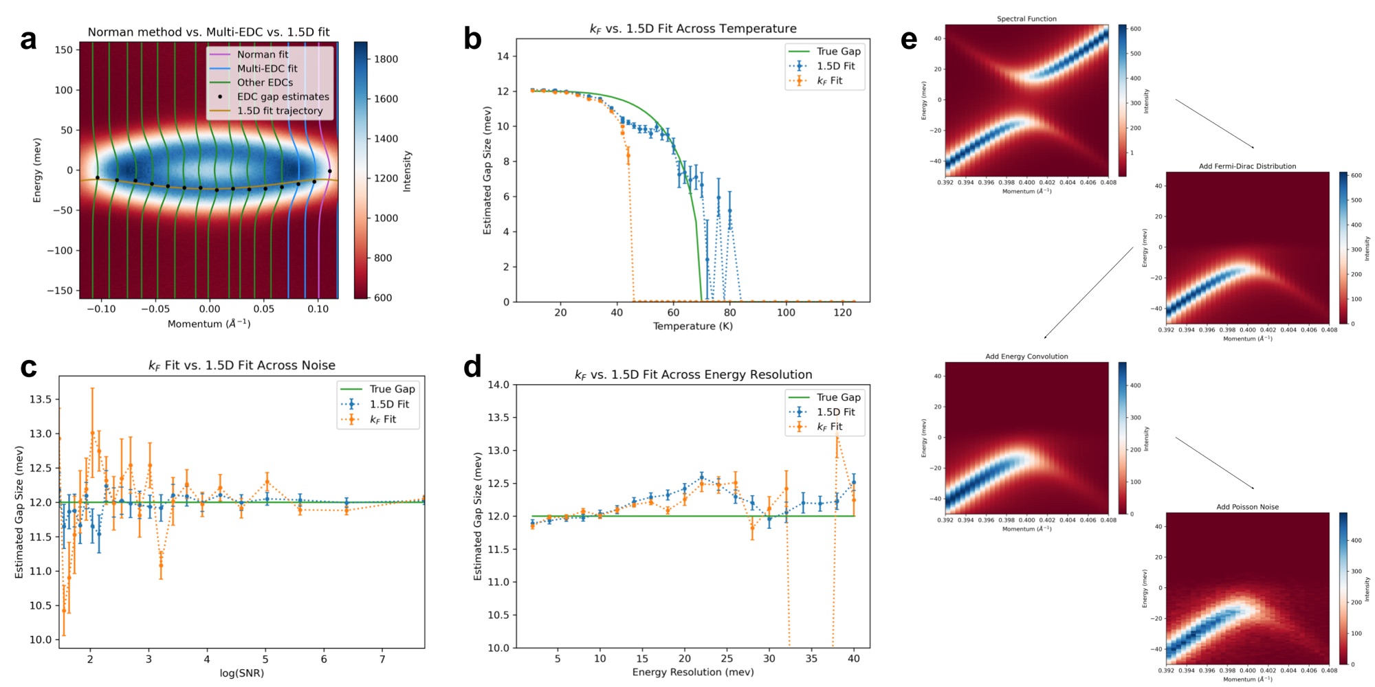
k_F fit on simulated spectra with a known gap. (a) A single simulated spectrum with the Norman fit (magenta), the multi-EDC fit (blue), the per-EDC gap estimates (black dots), and the 1.5D fit trajectory (gold) overlaid. (b) Estimated gap versus temperature: the 1.5D fit (blue) tracks the true gap (green) smoothly down to T_c, while the k_F fit (orange) collapses to zero early once the gap drops below resolution. (c) Gap versus noise and (d) gap versus energy resolution: both fits agree for a large 12 meV gap, but the k_F fit’s estimate scatters far more as conditions worsen. (e) The simulation pipeline: spectral function → Fermi–Dirac distribution → energy convolution → Poisson noise, the same chain a real analyzer imposes.Real data, and where it breaks
On three real Bi-2212 samples, an anti-node cut, a far-from-node cut, and a near-node cut, each scanned from below to above the critical temperature, the payoff showed up where the theory said it should. For the far-from-node and near-node samples, where the gap dips below resolution near T_c, the conventional fit’s gap-vs-temperature curve jumped around with large error bars, while the 1.5D fit traced a smooth, physical gap closure.
But it doesn’t fail gracefully. Most gap-extraction methods err conservative: they miss gaps that are really there. The 1.5D fit leans the other way: by design it’s hunting for faint sub-resolution gaps, so it’s more prone to “finding” a gap that isn’t there. On the anti-node sample, which has an unusually flat dispersion (exactly the case where Eq. 3 is hardest to pin down), the conventional fit actually did better, and the 1.5D fit reported false gaps above T_c where the real gap is zero. A flat band gives the dispersion fit too little curvature to work with, and a conventional k_F fit is correspondingly more forgiving of errors there.
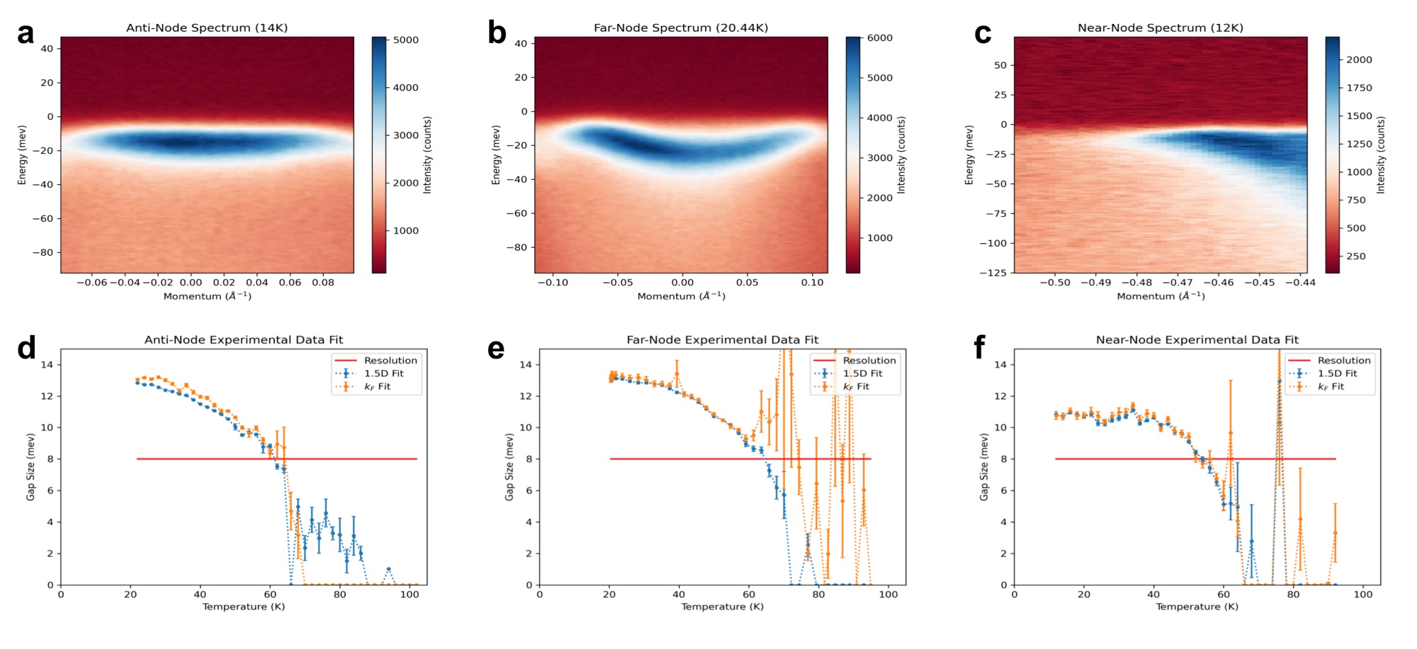
k_F fit (orange), and the 8 meV energy-resolution line (red). Below that line the gap is sub-resolution. For the far-node (e) and near-node (f) cuts the 1.5D fit closes smoothly through T_c while the k_F fit scatters. On the flat anti-node cut (d) the ranking reverses: the k_F fit closes cleanly while the 1.5D fit reports spurious gaps above T_c, its main failure mode.The method does one real thing well: below the resolution limit, reading the gap off the band’s dispersion is meaningfully more stable than fitting a single blurred slice. It also trades one blind spot for another: the conventional fit misses faint gaps, and this one occasionally invents them, especially on flat bands. It’s an improvement inside a specific niche, not a universal replacement. We drafted a fuller writeup, weighed that narrow win against the false-gap failure mode and where the field was heading (full-2D and CNN-based extraction), and decided to shelve it rather than push to publication.
The code
It’s a single-author Python research codebase (NumPy, SciPy, and lmfit) built up over 2021–2023: the Norman spectral-function model, symmetrization that cancels the Fermi cutoff, resolution convolution with Poisson-weighted fitting, the two-round trajectory fit above, and an F-test-based model-selection step for the nuisance parameters that vary with momentum. The source is on GitHub. Fair warning: it’s research code, not a package. It’s wired to my old data paths and the specific ARPES maps rather than built to run turnkey, so it’s there to read the method, not to pip install.
Spectral-function model from M. R. Norman, M. Randeria, H. Ding & J. C. Campuzano, Phenomenology of the low-energy spectral function in high-Tc superconductors, Phys. Rev. B 57, R11093 (1998); Bogoliubov-quasiparticle picture from H. Matsui et al., Phys. Rev. Lett. 90, 217002 (2003). Advised by Prof. Yu He (Yale Applied Physics). The 2021 poster took 2nd place at a Berkeley Advanced Light Source user meeting.